14 Introduction to Regression Analysis
This chapter is under heavy development and may still undergo significant changes.
As a reminder, we said that epidemiology is usually defined as something like, “the study of the occurrence and distribution of health-related states or events in specified populations, including the study of the determinants influencing such states, and the application of this knowledge to control the health problems.”1 In previous chapters, we reviewed some of the ways we can measure the occurrence of those states or events. We also reviewed measures of association – measures in the average change in the probability of a health state or event across levels of some other exposure, or exposures, of interest. In this part of the book, we are going to add another useful tool to our toolbox for measuring occurrence and association – regression analysis.
If you haven’t heard the word “regression” before, its meaning probably isn’t self-evident. It may even sound weird or intimidating. Formally, regression can be defined in the following way.
“A regression of a variable Y on another variable, say an exposure X, is a function that describes how some feature of the distribution of Y changes across population subgroups defined by values of X.”3
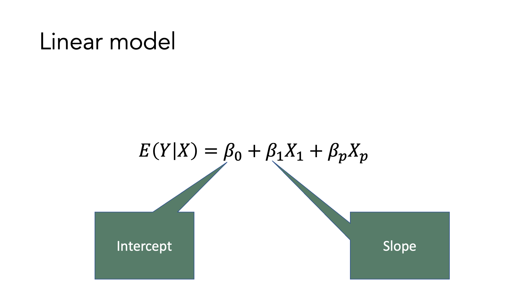
As an equation, the statement above can be written like this:
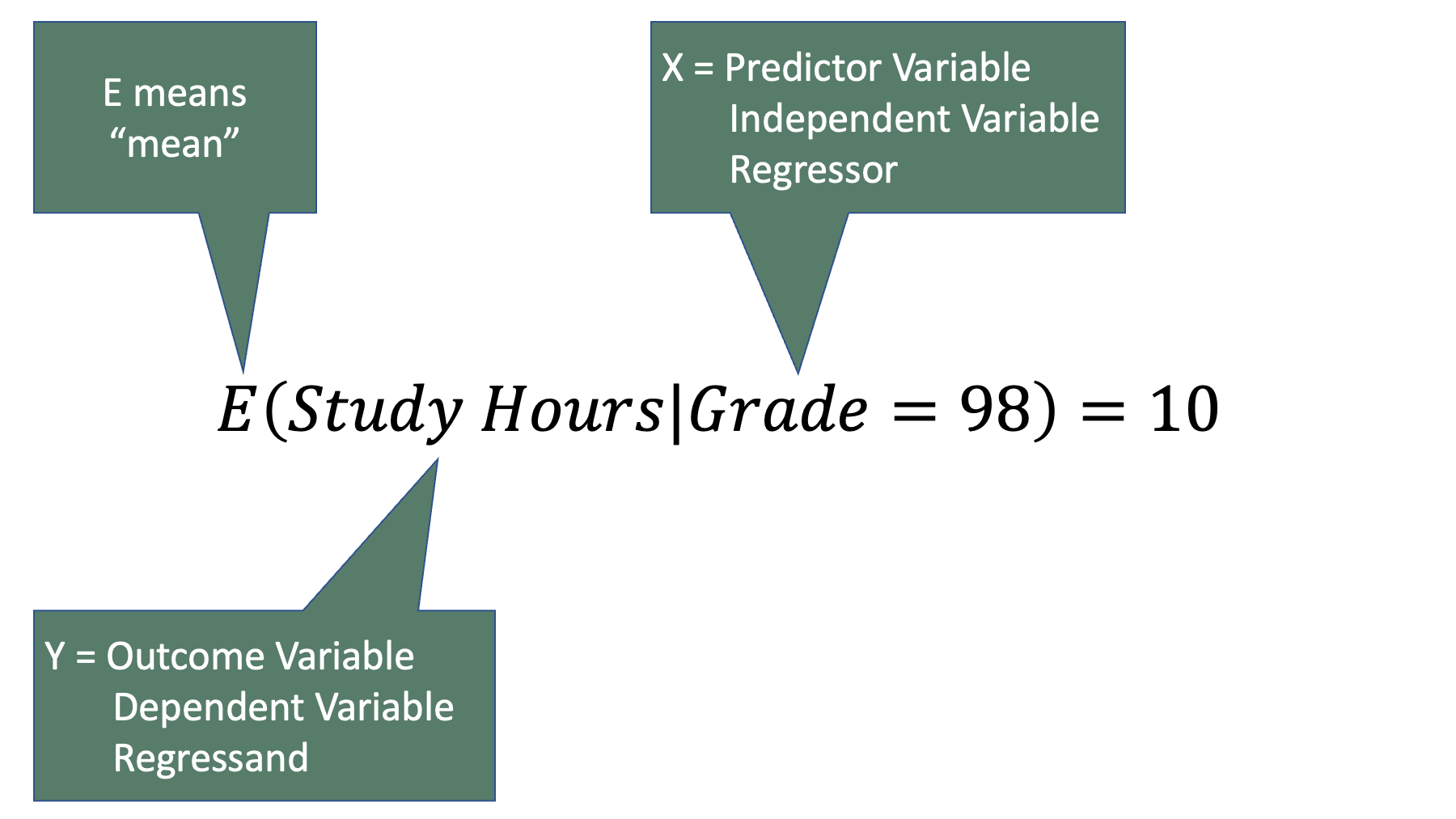
Where, means “expected value” or “average” of whatever is inside of the parentheses. So, we could articulate this equation in words as, The average value of Y when the variable X has a specific value, x.
For example, we could write a statement like “the average grade in an introduction to epidemiology class is 95” as . Further, we could write a statement like “The average grade in an introduction to epidemiology class is a 98 among people who study 10 hours per week” as .
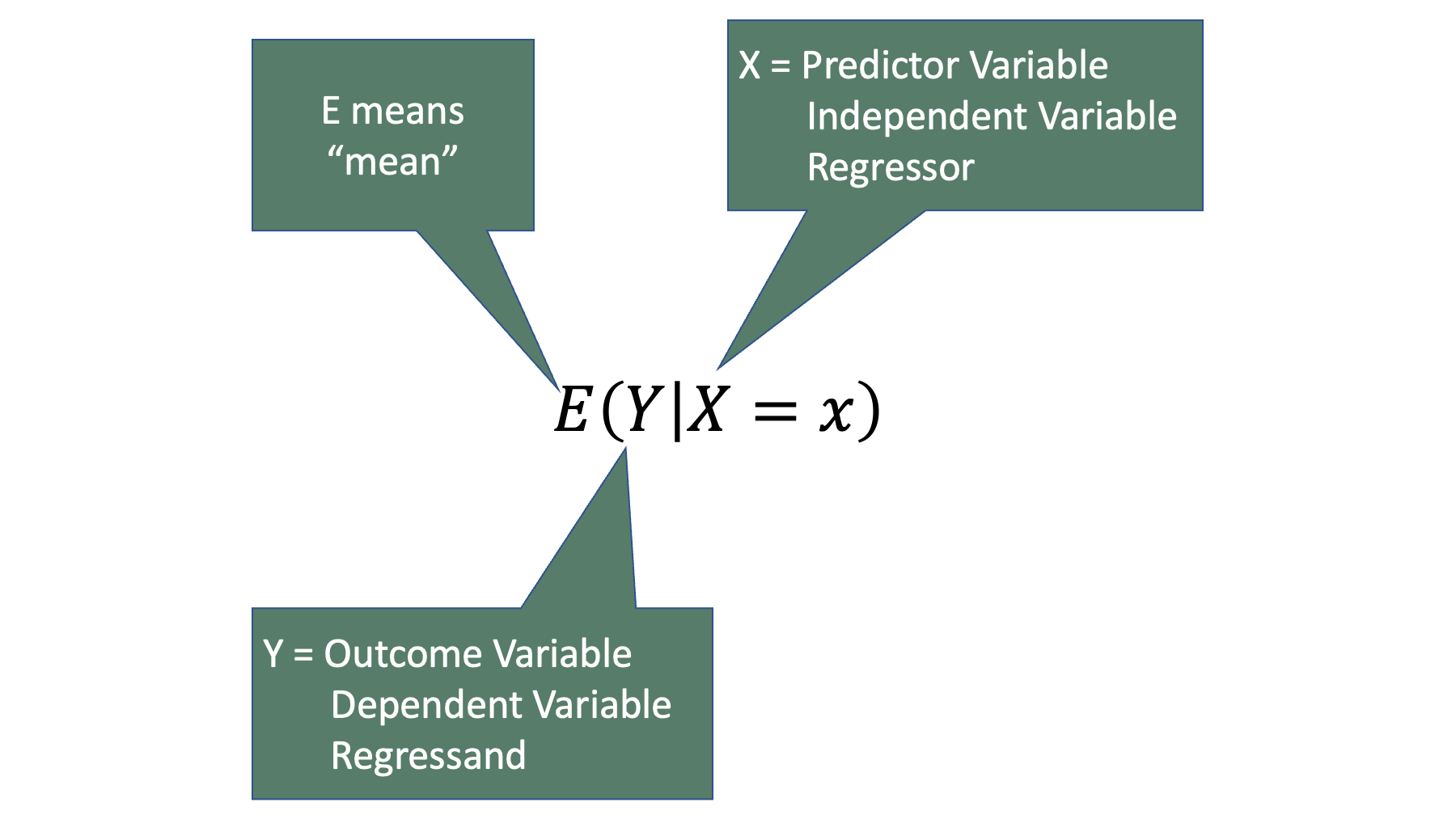
Notice that the term is commonly called the outcome variable, dependent variable, or the regressand. Similarly, the term is commonly called the predictor variable, independent variable, or the regressor. We will try to use the terms regressand and regressor in this book – even though they are not the most commonly used terms and probably have no intuitive meaning to the vast majority of you. In fact, we will use those terms precisely because they probably don’t have any intuitive meaning to you. And because they don’t have any intuitive meaning to you, it is unlikely that they will invoke any of the preconceived notions in your mind, which may or may not be accurate, that the other terms would. For example, “outcome variable” and “dependent variable” both imply a cause-and-effect relationship for many people. But as we discussed in the measures of association chapter, associations frequently exist between two variables even when there isn’t a cause and effect relationship between two variables (i.e., spurious correlations). Conversely, the terms “regressand” and “regressor” don’t tend to imply a preference for causal, or even temporal, relationships. For example, let’s plug some example variables into the regression equation from above. Specifically, let’s make study hours the regressand and grade the regressor.
The equation above is a totally valid, and possibly even useful, model of the relationship between study hours and grades, but it is not a valid causal model. How do we know that? Well, most of us intuitively know that our grade in this class (as opposed to a previous class) does not cause the number of hours we study. It couldn’t possibly. The studying occurs before we ever get the grade. Further, it doesn’t even really make sense to say that our grade in this class predicts the number of hours we will study. Again, the studying occurs before we ever get the grade. In this case, our intuition will help prevent us from making inaccurate statements about the results of regression analysis (i.e., grade causes study hours), but that won’t always be true. Causal and temporal relationships won’t always be so obvious. In those cases, the results can sometimes inadvertently invite us to make statements about the relationship between the variables that we can’t really justify.
14.1 Generalize linear models
So far, we’ve been discussion regression as though it is a singular thing. In practice, regression models can take many different forms. Many of the most commonly used forms fall into a category of regression models called Generalized Linear Models, or GLMs for short. GLMs are generally made up of three components:
A linear function that describes the average value of the regressand of the outcome.
A transformation of the mean of the regressand (the link function).
An assumed distribution of the regressand (from the exponential family).
The table below gives the name, generalized model form (equation), link function, and assumed distribution of the regressand for linear regression, logistic regression, Poisson regression, and Cox proportional hazards regression models. Together, these four models represent the majority of the generalized linear models used in epidemiology.
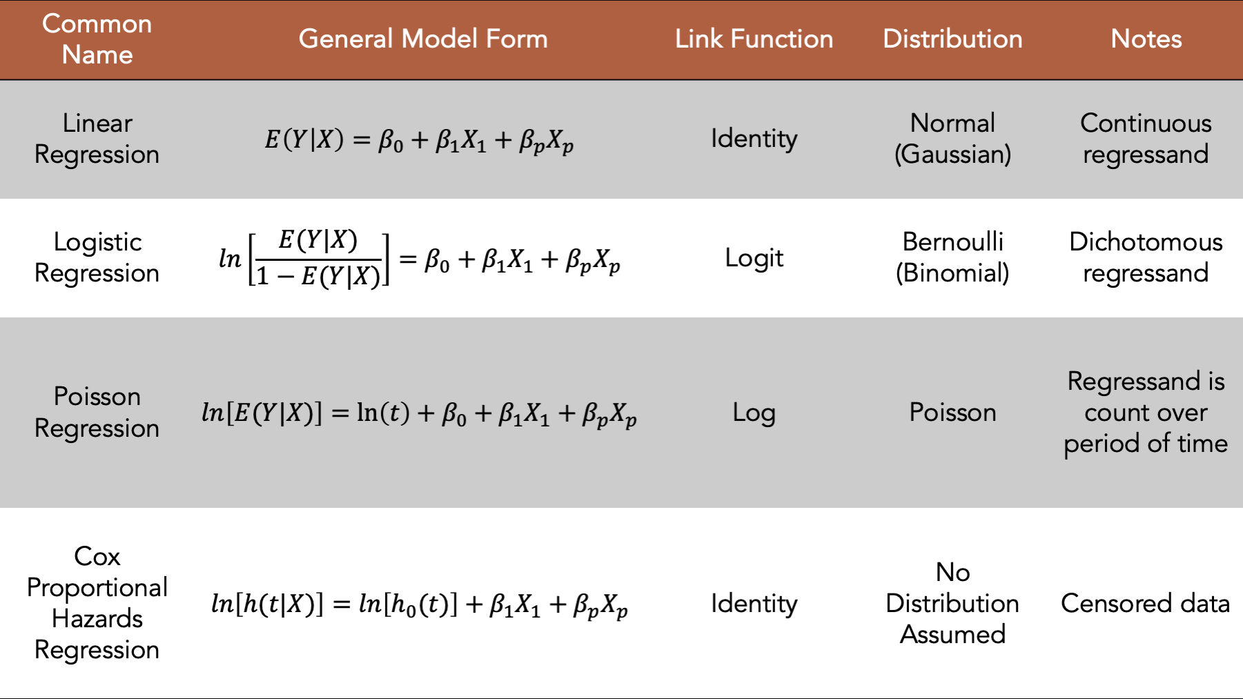
Figure 14.1: Four commonly used generalized linear models.
However, before we jump into building linear regression models in R, let’s review a concept that many people learned early in the algebra curriculum – the slope-intercept form of the equation of a straight line.
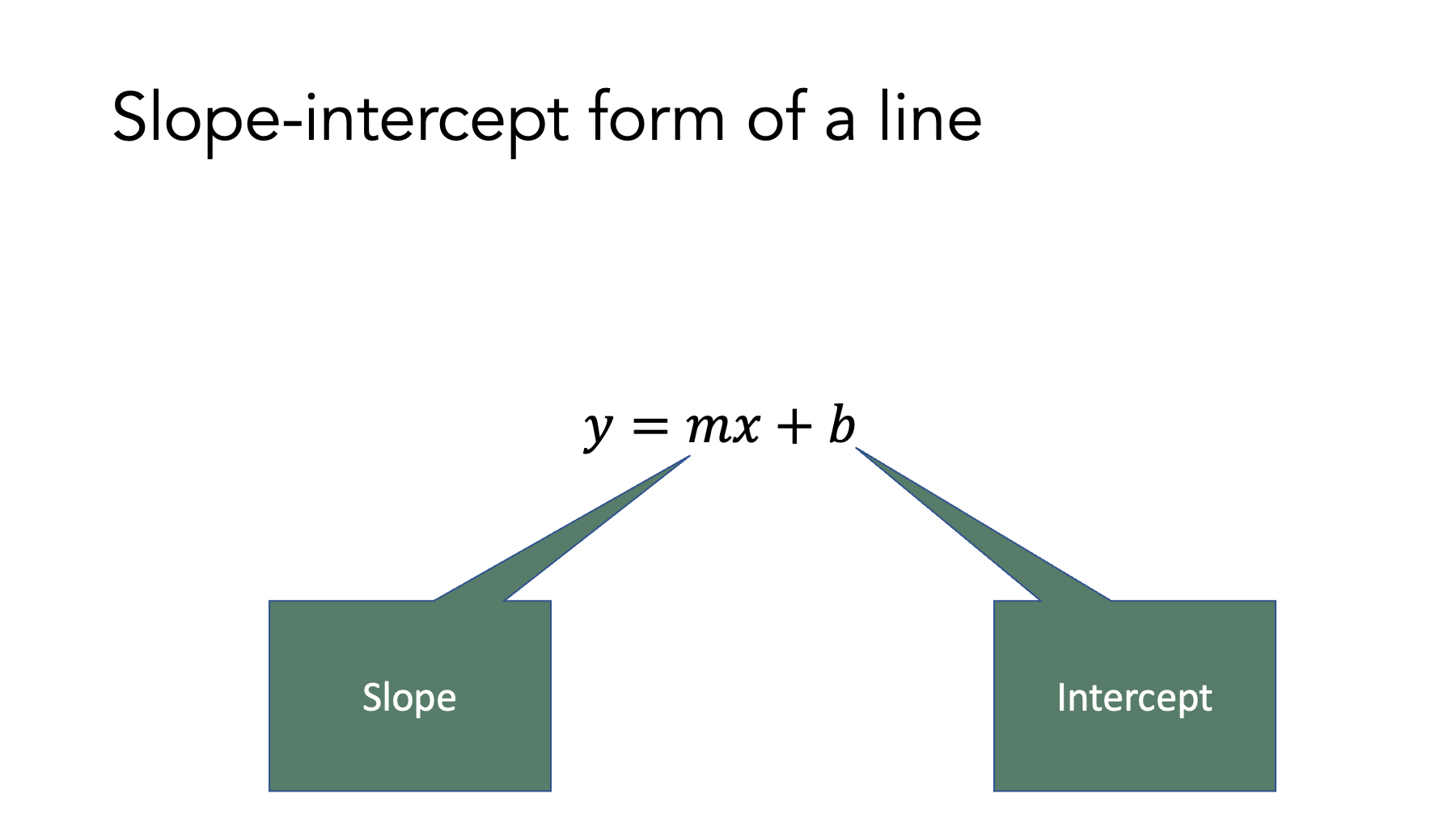
Do you remember this equation? It is a specific form of a linear equation that we can use to determine the value of when we know the value of , the intercept of the line (i.e., the value of when is zero), and the slope of the line.
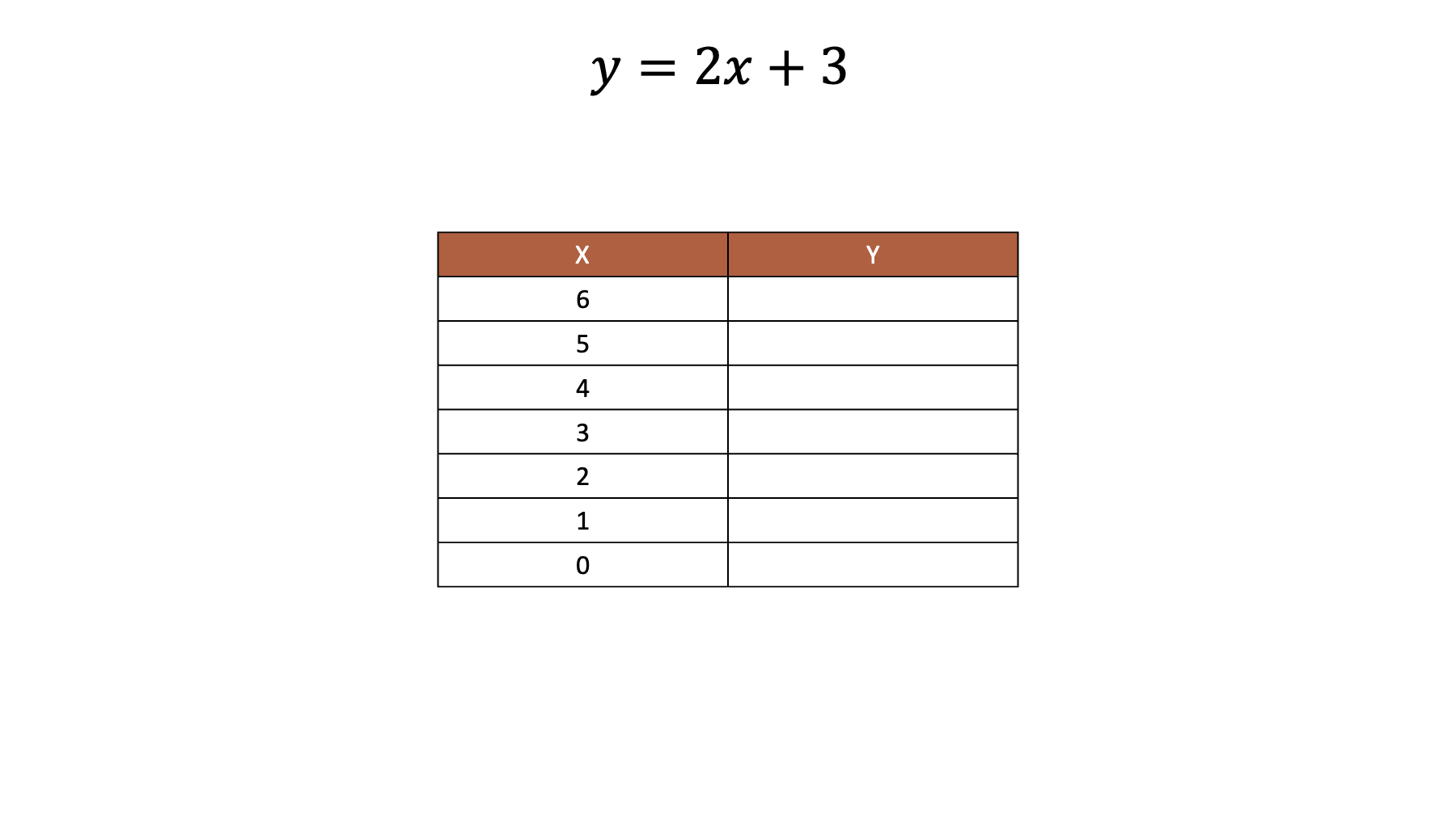
For example, let’s say that we have the following equation and values of .
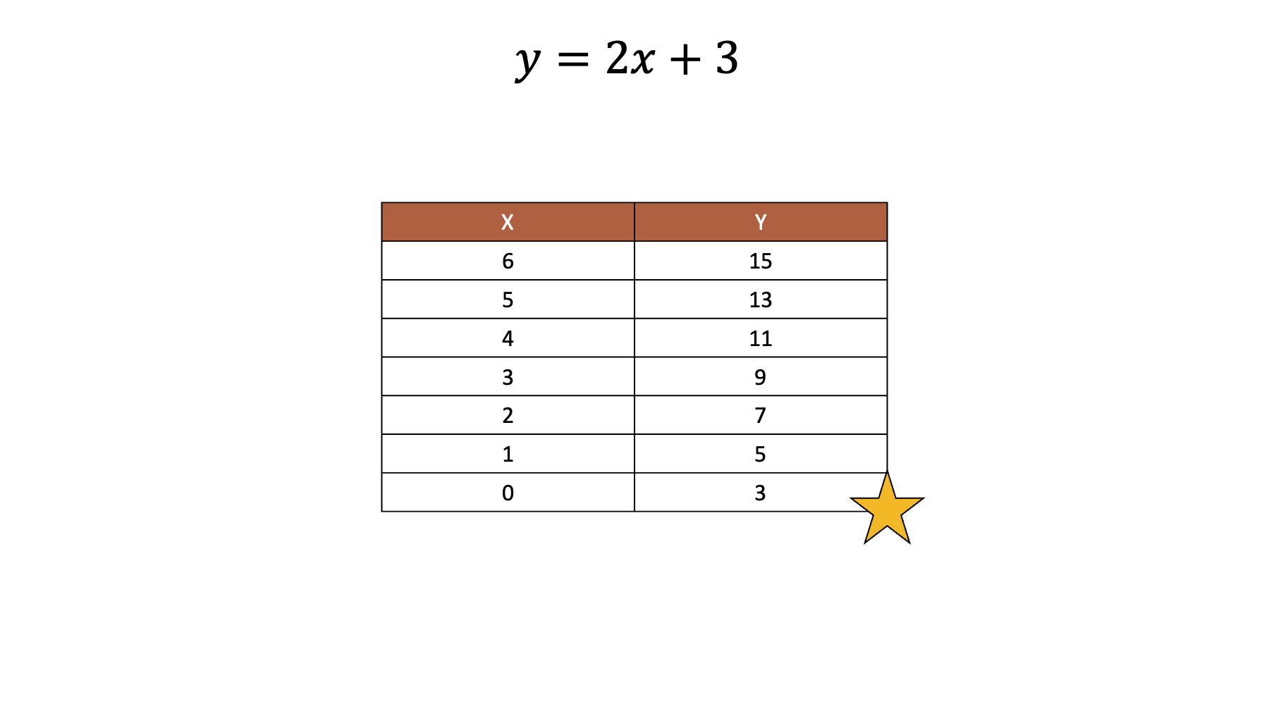
Armed with that information, we can easily work out the values of .
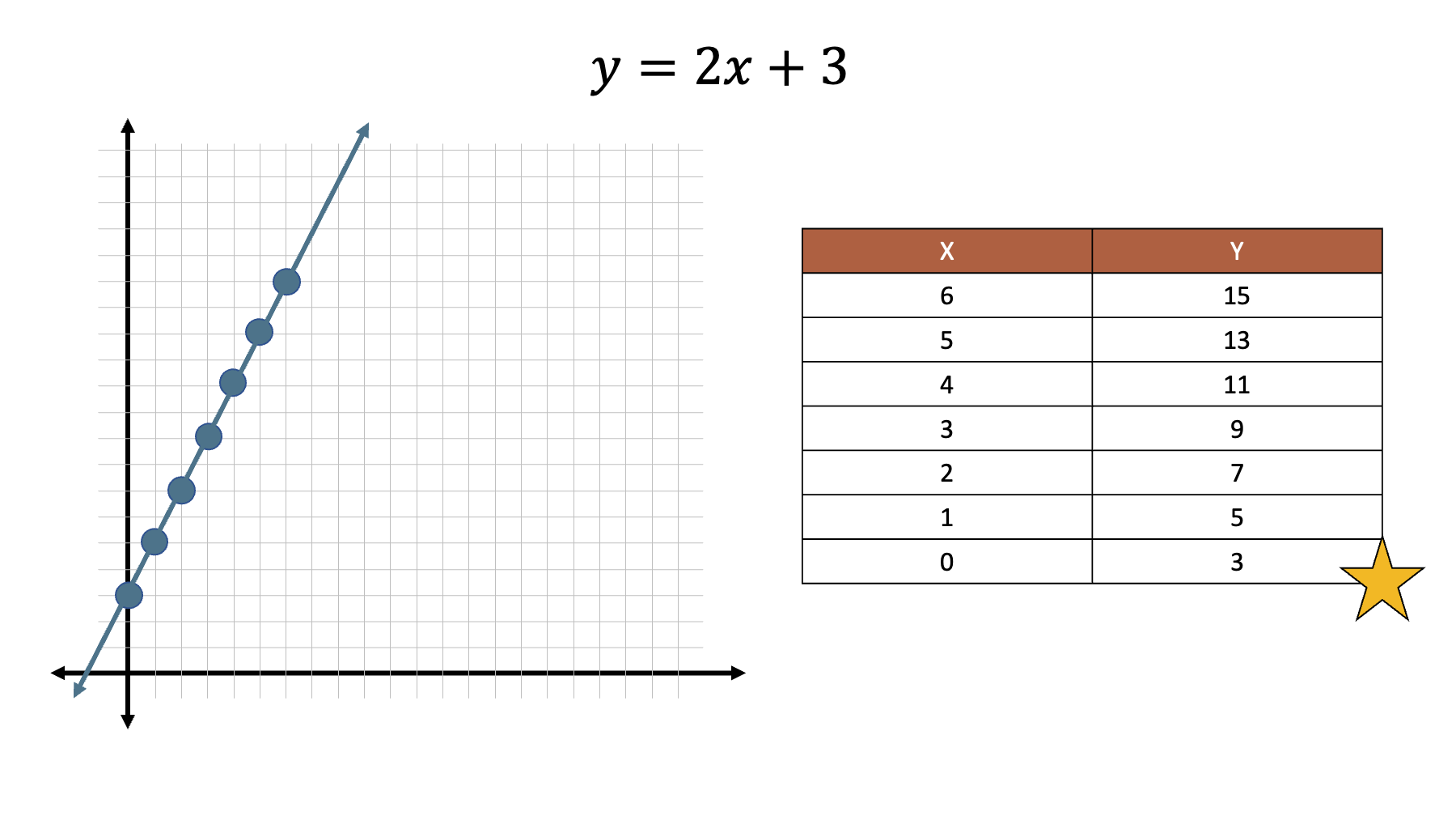
And when we plot those values on a line.
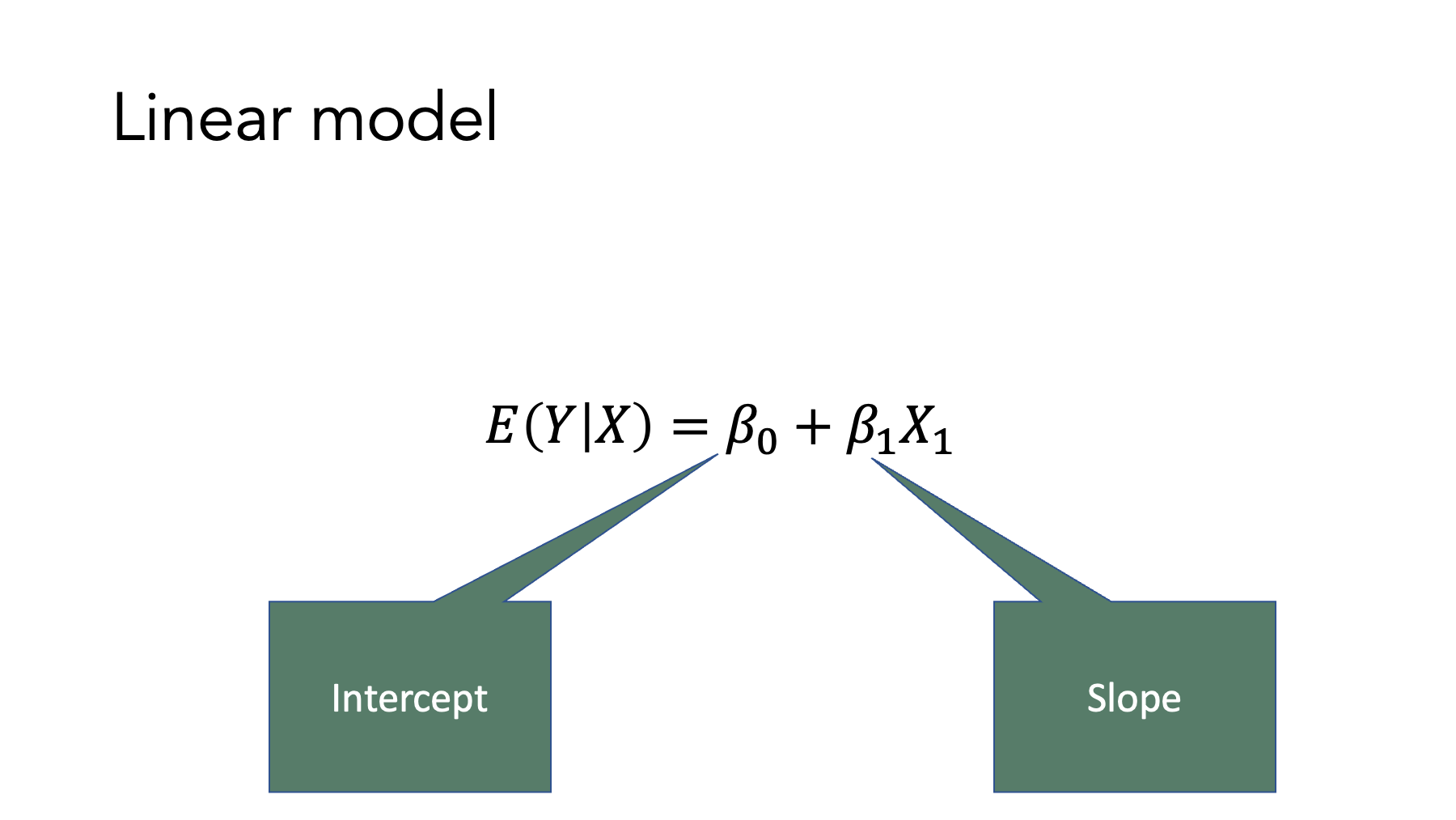
Now, look at the general model form of the equations in table 14.1. Do you see the similarities? We still have an value, a slope, and an intercept. And they are all interpreted similarly to how we would interpret the analogous terms in the slope-intercept formula. So, when we fit generalized linear regression models to our data, we will constrain the values predicted by our models to fall on a straight line (after doing some type of mathematical transformation in all cases except the linear model). Of course, real-world values very rarely fall on a perfectly straight line. Therefore, our regression models will also include an “error” term (not shown) to account for the differences between the values our model predicts – the ones that fall perfectly on the line – and the actual values in our data. Nonetheless, the basic concept is strikingly similar to the slope-intercept form of a line that you likely learned many years ago.
14.1.1 The glm function
In R, we fill one of our generalized linear models to our data using the glm() function. Actually, this isn’t totally true. We the Cox proportional hazard model is fit to data using a different function. The Cox proportional hazards model is technically a generalized linear model, but it has some important differences from the other three shown above. Therefore, we will introduce linear, logistic, and Poisson regression only in this chapter. We will discuss the Cox proportional hazards model later as part of our broader discussion of survival analysis.
Let’s start by simulating some data and then fitting a model to that data. After viewing a complete working example, we will break down the code and discuss it in greater detail.
The code below simulates a data frame that contains the age (age) and weekly minutes of physical activity (phys_act) for a sample of 100 people. We add comments to the code below to help you get a sense for how the values are generated. But please skip over the code if it feels distracting or confusing, as it is not the primary object of our interest right now.
# Set the seed for the random number generator so that we can reproduce our results
set.seed(123)

# Simulate a sample of 100 people
# Include measures of physical activity and age
physical_activity_age <- tibble(
  # Create participant ids
  id = 1:100,
  # Sample ages between 18 and 100
  age = sample(18:100, 100, TRUE),
  # Center age at 18
  age_c = age - 18,
  # Create term that quantifies the change in the mean value of weekly minutes
  # of physical activity for each additional year of age plus some random
  # variation.
  beta_1 = rnorm(100, mean = -2, sd = 0.5),
  # Set the value for weekly minutes of physical activity as 140 at age 18,
  # declining by beta_1 for each additional year of age after 18 (age_c).
  phys_act = 140 + (beta_1 * age_c)
)

# Print the value stored in physical_activity_age to the screen
physical_activity_age
## # A tibble: 100 × 5
## id age age_c beta_1 phys_act
## <int> <int> <dbl> <dbl> <dbl>
## 1 1 48 30 -1.68 89.7
## 2 2 96 78 -2.11 -24.6
## 3 3 68 50 -1.83 48.3
## 4 4 31 13 -1.45 121.
## 5 5 84 66 -1.78 22.4
## 6 6 59 41 -2.16 51.3
## 7 7 67 49 -1.43 70.1
## 8 8 60 42 -1.50 76.9
## 9 9 31 13 -1.73 118.
## 10 10 42 24 -1.88 94.9
## # ℹ 90 more rowsNext, let’s fit a generalized linear model to the data we simulated above.
##
## Call:  glm(formula = phys_act ~ age, family = gaussian(link = "identity"),
##     data = physical_activity_age)
##
## Coefficients:
## (Intercept)          age
##     176.171       -1.993
##
## Degrees of Freedom: 99 Total (i.e. Null);  98 Residual
## Null Deviance:       268600
## Residual Deviance: 47170     AIC: 905.4
If you already know how to interpret these results, that’s great! If not, don’t worry. We will learn how to interpret them soon, but not now. Right now, we are just interested in the R code we used to produce these results. In general, we will need to pass the following the following information to the glm() function when fitting a generalized linear model to our data in R:
glm(
  # formula = The regression formula Y ~ X
  # family  = The distribution family and link function
  # data    = The data frame containing the data we want to fit the model to
)
First, we pass a formula the glm() function takes the form Y ~ X, where Y is the regressand, tilde (~) means “equals”, and X is the regressor. In our example above, we had data on age (age) and weekly minutes of physical activity (phys_act). We wanted to model physical activity as the regressand and age as the regressor, so we passed phys_act ~ age to the formula argument. This formula is very similar to the general model form shown in table 14.1 above. However, the general model form shown in table 14.1 shows the regressand with the link function already applied. For example, ln[E(Y|X)] or ln[E(phys_act|age)] instead of just E(Y|X) or E(phys_act|age). In the glm() function, we tell R to what link function to apply to Y using the family argument (discussed next).
Second, we pass one of the following distribution family and link functions to the family argument of the glm() function. In the example above, we passed the gaussian(link = "identity") to the family argument to fit a linear regression model to our data.
| Regression Model | Distribution Family | Link Function | Combined Form |
|---|---|---|---|
| Linear | gaussian() | link = “identity” | gaussian(link = “identity”) |
| Logistic | binomial() | link = “logit” | binomial(link = “logit”) |
| Poisson | poisson() | link = “log” | poisson(link = “log”) |
Third, we enter the name of the data frame we want to pass to our regression model in the data argument of the glm() function. In the example above, we passed physical_activity_age to the data argument.
In this example, we fit a linear regression model to our simulated data, but the syntax is nearly identical for other generalized linear models that we fit with R’s glm() function. We just change the formula to reflect the variables we are interested in modeling and change the distribution and link function to match the form of relationship we want to model. When to change them, what to change them to, and how to interpret the results we get from our models will be the topic of the rest of this part of the book.
14.2 Regression intuition
In the sections above, we formally defined regression analysis and we introduced R’s glm() function – a function we an use to fit generalized linear models to our data. Now, let’s walk through another example to help us develop our intuition about what is happening “under the hood” in regression models. For this example, we want to regress diabetes (0 = Negative, 1 = Positive) on family history of diabetes (0 = No, 1 = Yes), to investigate the relationship between diabetes and family history of diabetes in our data.
# Simulate a sample of 698 people
# Include measures of family history of diabetes (0 = No, 1 = Yes) and diabetes
# (0 = Negative, 1 = Positive)
diabetes <- tidyr::expand_grid(
  family_history = c(1, 0),
  diabetes       = c(1, 0)
) %>%
  mutate(count = c(58, 196, 63, 381)) %>%
  tidyr::uncount(count)

# Print the value stored in diabetes to the screen
diabetes
## # A tibble: 698 × 2
## family_history diabetes
## <dbl> <dbl>
## 1 1 1
## 2 1 1
## 3 1 1
## 4 1 1
## 5 1 1
## 6 1 1
## 7 1 1
## 8 1 1
## 9 1 1
## 10 1 1
## # ℹ 688 more rowsRemember, in the frequentist view, the regression of a variable on another variable is the function that describes how the average (mean) value of changes across population subgroups defined by values of .3 And for dichotomous variables that take the values 0 and 1 only, the mean of the vector of values is equal to the proportion of 1’s. For example, let’s say we have a vector of 5 numbers – 3 ones and 2 zeros.
The mean of those numbers will be:
And the proportion of ones in the vector will be:
With that in mind, the mean value of diabetes across subgroups defined by family_history are:
## # A tibble: 2 × 11
##   response_var group_var      group_cat     n  mean    sd    sem   lcl   ucl   min   max
##   <chr>        <chr>              <dbl> <int> <dbl> <dbl>  <dbl> <dbl> <dbl> <dbl> <dbl>
## 1 diabetes     family_history         0   444  0.14  0.35 0.0166  0.11  0.17     0     1
## 2 diabetes     family_history         1   254  0.23  0.42 0.0264  0.18  0.28     0     1
The mean value of diabetes across subgroups defined by family_history are 0.14 when family_history equals 0 and 0.23 when family_history equals 1. Additionally, the proportion of people with diabetes across subgroups defined by family_history are:
## # A tibble: 4 × 6
##   row_var        row_cat col_var  col_cat     n percent_row
##   <chr>          <chr>   <chr>    <chr>   <int>       <dbl>
## 1 family_history 0       diabetes 0         381        85.8
## 2 family_history 0       diabetes 1          63        14.2
## 3 family_history 1       diabetes 0         196        77.2
## 4 family_history 1       diabetes 1          58        22.8
Take a look at the percentage of people with family history of diabetes who have diabetes (22%) and the percentage of people without family history of diabetes who have diabetes (14%). You should notice that it is the same as the subgroup means (multiplied by 100 because they are percentages).
This illustrates an important property: “When the regressand Y is a binary indicator (0, 1) variable, is called a binary regression, and this regression simplifies in a very useful manner. Specifically, when Y can be only 0 or 1 the average equals the proportion of population members who have Y=1 among those who have X=x.”3
Now, let’s fit a linear regression model to this data.
##
## Call:  glm(formula = diabetes ~ family_history, family = gaussian(link = "identity"),
##     data = diabetes)
##
## Coefficients:
##    (Intercept)  family_history
##        0.14189         0.08645
##
## Degrees of Freedom: 697 Total (i.e. Null);  696 Residual
## Null Deviance:       100
## Residual Deviance: 98.82     AIC: 622.3
And here is how we can interpret the coefficients from the model:
Intercept: The mean value of
diabeteswhenfamily_historyis equal to zero. Notice, that this value (0.14) is the same value we estimated above for the mean ofdiabeteswhenfamily_historyis equal to zero and for the proportion of people with diabetes whenfamily_historyis equal to zero.family_history: The average change in
diabetesfor each one-unit increase infamily_history. In this case,family_historycan only take two values – zero and one. So, there can be only one one-unit increase – from zero to one. So, the value ofdiabeteswhenfamily_historyis equal to zero is 0.14189 and the value ofdiabeteswhenfamily_historyis equal to one increase by 0.08645 to 0.14189 + 0.08645 = 0.22834. Does that value look familiar? It is the same value we estimated above for the mean ofdiabeteswhenfamily_historyis equal to one and for the proportion of people with diabetes whenfamily_historyis equal to one.
Hopefully, this illustration has increased your comfort level with regression analysis. It’s just an extension of the simpler methods we have previously learned about. However, regression models can easily be extended to accommodate analyzing the average change in across levels of multiple variables simultaneously – multivariable (not to be confused with multivariate) regression. This is one of the primary advantages to using regression analysis instead of many of the simpler methods we’ve learned about. Imagine how messy the mean tables and/or frequency tables would get if we had 10 regressor variables instead of one.
As an important side note, we will not typically fit a linear regression to data with a binary regressand as we did above. This example was only meant to give you a feel the relationship between regression coefficients and some of the other methods we’ve learned that tend to be more intuitively easy to understand. In the following chapter, we will take a look at a more realistic example of using linear regression to model a continuous regressand.